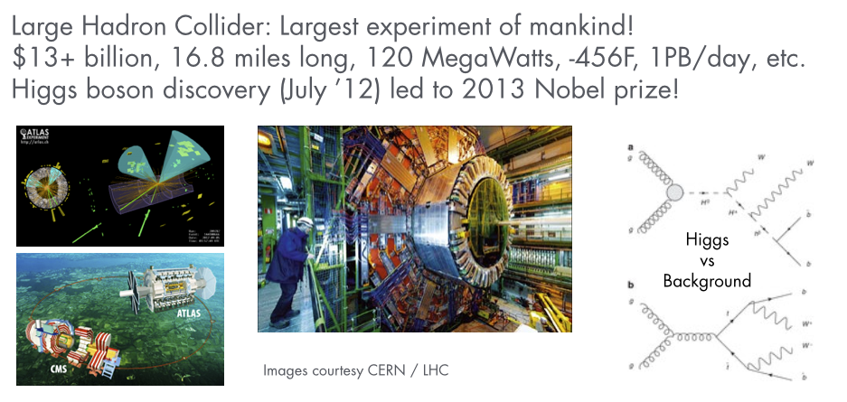
Higgs Particle Discovery with H2O Deep Learning
This tutorial shows how H2O can be used to classify particle detector events into Higgs bosons vs background noise. This file is both valid R and markdown code.
HIGGS dataset and Deep Learning
We use the UCI HIGGS dataset with 11 million events and 28 features (21 low-level features and 7 humanly created non-linear derived features). In this tutorial, we show that (only) Deep Learning can automatically generate these or similar high-level features on its own and reach highest accuracies from just the low-level features alone, outperforming traditional classifiers. This is in accordance with a recently published Nature paper on using Deep Learning for Higgs particle detection. Remarkably, Deep Learning also won the Higgs Kaggle challenge on the full set of features.
Start H2O, import the HIGGS data, and prepare train/validation/test splits
Initialize the H2O server (enable all cores)
library(h2o)
h2oServer <- h2o.init(nthreads=-1)
Import the data: For simplicity, we use a reduced dataset containing the first 100k rows.
homedir <- "/data/h2o-training/higgs/"
TRAIN = "higgs.100k.csv.gz"
data_hex <- h2o.importFile(h2oServer, path = paste0(homedir,TRAIN), header = F, sep = ',', key = 'data_hex')
For small datasets, it can help to rebalance the dataset into more chunks to keep all cores busy
data_hex <- h2o.rebalance(data_hex, chunks=64, key='data_hex.rebalanced')
Prepare train/validation/test splits: We split the dataset randomly into 3 pieces. Grid search for hyperparameter tuning and model selection will be done on the training and validation sets, and final model testing is done on the test set. We also assign the resulting frames to meaningful names in the H2O key-value store for later use, and clean up all temporaries at the end.
random <- h2o.runif(data_hex, seed = 123456789)
train_hex <- h2o.assign(data_hex[random < .8,], "train_hex")
valid_hex <- h2o.assign(data_hex[random >= .8 & random < .9,], "valid_hex")
test_hex  <- h2o.assign(data_hex[random >= .9,], "test_hex")
h2o.rm(h2oServer, grep(pattern = "Last.value", x = h2o.ls(h2oServer)$Key, value = TRUE))
The first column is the response label (background:0 or higgs:1). Of the 28 numerical features, the first 21 are low-level detector features and the last 7 are high-level humanly derived features (physics formulae).
response = 1
low_level_predictors = c(2:22)
low_and_high_level_predictors = c(2:29)
Establishing the baseline performance reference with several H2O classifiers
To get a feel for the performance of different classifiers on this dataset, we build a variety of different H2O models (Generalized Linear Model, Random Forest, Gradient Boosted Machines and DeepLearning). We would like to use grid-search for hyper-parameter tuning with N-fold cross-validation, and we want to do this twice: once using just the low-level features, and once using both low- and high-level features.
First, we source a few helper functions that allow us to quickly compare a multitude of binomial classification models, in particular the h2o.fit() and h2o.leaderBoard() functions. Note that these specific functions require variable importances and N-fold cross-validation to be enabled.
source("~/h2o-training/tutorials/advanced/binaryClassificationHelper.R.md")
The code below trains 60 models (2 loops, 5 classifiers with 2 grid search models each, each resulting in 1 full training and 2 cross-validation models). A leaderboard scoring the best models per h2o.fit() function is displayed.
N_FOLDS=2

for (preds in list(low_level_predictors, low_and_high_level_predictors)) {
  data = list(x=preds, y=response, train=train_hex, valid=valid_hex, nfolds=N_FOLDS)

  models <- c(
    h2o.fit(h2o.glm, data,
            list(family="binomial", variable_importances=T, lambda=c(1e-5,1e-4), use_all_factor_levels=T)),
    h2o.fit(h2o.randomForest, data,
            list(type="fast", importance=TRUE, ntree=c(5), depth=c(5,10))),
    h2o.fit(h2o.randomForest, data,
            list(type="BigData", importance=TRUE, ntree=c(5), depth=c(5,10))),
    h2o.fit(h2o.gbm, data,
            list(importance=TRUE, n.tree=c(10), interaction.depth=c(2,5))),
    h2o.fit(h2o.deeplearning, data,
            list(variable_importances=T, l1=c(1e-5), epochs=1, hidden=list(c(10,10,10), c(100,100))))
  )
  best_model <- h2o.leaderBoard(models, test_hex, response)
  h2o.rm(h2oServer, grep(pattern = "Last.value", x = h2o.ls(h2oServer)$Key, value = TRUE))
}
The output contains a leaderboard (based on validation AUC) for the models using low-level features only:
#                                        model_type train_auc validation_auc    important_feat tuning_time_s
#    DeepLearning_ba44837829dc8d1e h2o.deeplearning 0.6102486      0.6661170  C7,C3,C10,C11,C2      5.604354
#    GBM_8aad39d45442ed2418646fac4 h2o.gbm          0.6393795      0.6483558  C7,C2,C5,C10,C11      3.379146
#    DRF_b64f1aca48cfa9532f78408df h2o.randomForest 0.6358507      0.6439986  C7,C10,C2,C5,C11      4.423504
#    SpeeDRF_a40eda3fe25b1271b6be8 h2o.randomForest 0.5977397      0.6000200 C11,C7,C5,C10,C14      3.381785
#    GLMModel__9f5855ebfcb804a1664 h2o.glm          0.5907724      0.5893810  C5,C7,C14,C2,C10      1.422024
Note that training AUCs are based on cross-validation.
When using both low- and high-level features, the AUC values go up across the board:
#                                       model_type train_auc validation_auc     important_feat tuning_time_s
#    DeepLearning_a7cb0d0cc6f6fb8 h2o.deeplearning 0.7280887      0.7586982 C27,C29,C28,C24,C7      6.663959
#    GBM_bc87169c331b22e37339c643 h2o.gbm          0.7552951      0.7545594 C27,C29,C28,C7,C24      4.437348
#    DRF_b3572d5d088a043addcb3684 h2o.randomForest 0.7467827      0.7534905 C27,C29,C28,C24,C7      6.636395
#    SpeeDRF_ba048cb60c3aad567b17 h2o.randomForest 0.7274115      0.7301433 C27,C28,C29,C7,C24      5.516673
#    GLMModel__b59d95ace34a2979da h2o.glm          0.6827518      0.6764049 C29,C28,C27,C7,C24      1.523096
Clearly, the high-level features add a lot of predictive power, but what if they are not easily available? On this sampled dataset and with simple models from low-level features alone, Deep Learning seems to have an edge over the other methods indicating that it is able to create useful high-level features on its own.
Note: Every run of DeepLearning results in different results since we use Hogwild! parallelization with intentional race conditions between threads. To get reproducible results at the expense of speed for small datasets, set reproducible=T and specify a seed.
Build an improved Deep Learning model on the low-level features alone
With slightly modified parameters, it is possible to build an even better Deep Learning model. We add dropout/L1/L2 regularization and increase the number of neurons and the number of hidden layers. Note that we don't use input layer dropout, as there are only 21 features, all of which are assumed to be present and important for particle detection. We also reduce the amount of dropout for derived features. Note that the importance of regularization typically goes down with increasing dataset sizes, as overfitting is less an issue when the model is small compared to the data.
h2o.deeplearning(x=low_level_predictors, y=response, activation="RectifierWithDropout", data=train_hex,
                 validation=valid_hex, input_dropout_ratio=0, hidden_dropout_ratios=c(0.2,0.1,0.1,0),
                 l1=1e-5, l2=1e-5, epochs=20, hidden=c(200,200,200,200))
With this computationally slightly more expensive Deep Learning model, we achieve a nice boost over the simple models above: AUC = 0.7245833 (on validation)