Dimensionality Reduction of MNIST
This tutorial shows how to reduce the dimensionality of a dataset with H2O. We will use both PCA and Deep Learning. This file is both valid R and markdown code. We use the well-known MNIST dataset of hand-written digits, where each row contains the 28^2=784 raw gray-scale pixel values from 0 to 255 of the digitized digits (0 to 9).
Start H2O and load the MNIST data
Initialize the H2O server and import the MNIST training/testing datasets.
library(h2o)
h2oServer <- h2o.init(nthreads=-1)
homedir <- "/data/h2o-training/mnist/"
DATA = "train.csv.gz"
data_hex <- h2o.importFile(h2oServer, path = paste0(homedir,DATA), header = F, sep = ',', key = 'train.hex')
The data consists of 784 (=28^2) pixel values per row, with (gray-scale) values from 0 to 255. The last column is the response (a label in 0,1,2,...,9).
predictors = c(1:784)
resp = 785
We do unsupervised training, so we can drop the response column.
data_hex <- data_hex[,-resp]
PCA - Principle Components Analysis
Let's use PCA to compute the principal components of the MNIST data, and plot the standard deviations of the principal components (i.e., the square roots of the eigenvalues of the covariance/correlation matrix).
pca_model <- h2o.prcomp(data_hex)
plot(pca_model@model$sdev)
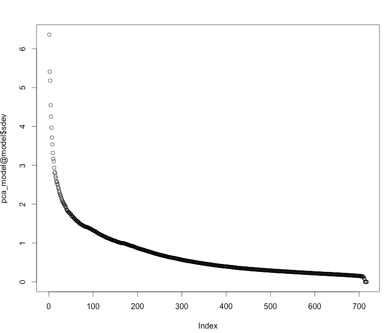
We see that the first 50 or 100 principal components cover the majority of the variance of this dataset.
To reduce the dimensionality of MNIST to its 50 principal components, we use the h2o.predict() function with an extra argument num_pc:
features_pca <- h2o.predict(pca_model, data_hex, num_pc=50)
summary(features_pca)
Deep Learning Autoencoder
ae_model <- h2o.deeplearning(x=predictors,
                            y=42, #ignored (pick any non-constant predictor)
                            data_hex,
                            activation="Tanh",
                            autoencoder=T,
                            hidden=c(100,50,100),
                            epochs=1,
                            ignore_const_cols = F)
We can now convert the data with the autoencoder model to 50-dimensional space (second hidden layer)
features_ae <- h2o.deepfeatures(data_hex, ae_model, layer=2)
summary(features_ae)
To get the full reconstruction from the output layer of the autoencoder, use h2o.predict() as follows
data_reconstr <- h2o.predict(ae_model, data_hex)
summary(data_reconstr)